Statistical power (SP) refers to the probability of rejecting a null hypothesis (a hypothesis of no difference) when it is actually false. When an organizational researcher retains (fails to reject) a false null hypothesis, he or she is likely to conclude, for example, that the organizational intervention did not positively affect productivity or that a selection test does not validly predict future job performance. Because an erroneous decision can have important practical implications, researchers would like to have adequate SP in order to be able to reject the null hypothesis when it is false. The amount of SP present when testing, say, the difference between two means or the relationship of two sets of values, is influenced by three factors: (a) the alpha level (a, or probability value) adopted for the statistical test, (b) the size of the sample used to obtain the means or correlation, and (3) the effect size (ES; or the magnitude of the difference or relationship). Before discussing these factors, a few words must be said about Type I and Type II errors in hypothesis testing.
Type I And Type II Errors
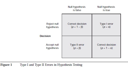
Figure 1 shows the interplay of accepting or rejecting a null hypothesis when it is actually true or false. A Type I error occurs when a null hypothesis (e.g., two variables that are not related or two subgroups that are not different) is rejected as being true, but it is actually true. A Type II error occurs when a null hypothesis is retained as being true, but it is actually not true. The probability of Type I error is denoted by alpha (a), and the probability of Type II error is denoted by beta (B). Statistical power—the probability of rejecting the null hypothesis when it is false— is equal to 1 minus the probability of a Type II error (1 – P).
In a statistical analysis, the likelihood that a Type I versus a Type II error will occur can be manipulated by adjusting the probability, or a level, for the statistical test. The most typical a value is .05. When a = .05, the rate of committing a Type I error is five times per 100 independent samples that might be compared. If a smaller value for a (e.g., .01) is chosen, the likelihood of committing a Type I error decreases, but the likelihood of a Type II error increases. Similarly, by increasing a (to a value greater than .05), we decrease the probability of a Type II error.
Factors Affecting Statistical Power
As noted previously, a, sample size, and ES play important roles in determining SP. According to Figure 1, SP is the converse of the probability of Type II error (SP = 1 – P). One way to decrease the likelihood of a Type II error is to increase a. Although there is nothing sacred about the commonly used a levels, one should be careful about increasing the a levels excessively. There are very few organizational interventions in which the treatment effect is truly zero; many treatments may have small effects but rarely zero effects. According to null hypothesis testing, Type I errors can only occur when the treatment effect is zero. Therefore, raising the a level without a good rationale is not recommended because the higher the a, the less rigorous the test of an effect, and the greater the chance of making a Type 1 error.
All else being equal, the bigger the sample size, the greater the SP. Therefore, one should obtain as big a sample as possible within prevailing practical constraints to ensure detection of a significant effect. Typically, obtaining a bigger sample is more time-consuming and costly. If the population correlation is .10, one would need a sample of 1,000 cases to have enough SP (say, SP = .80, which is generally considered acceptable) to detect it with a = .01, or a sample of more than 600 cases with a = .05.
Effect size is a way of quantifying the effectiveness of an organizational intervention. The bigger the ES, the greater the SP for detecting a significant organizational intervention effect for a given sample size and a level. A commonly used ES is the standardized mean difference, d, which can be calculated by dividing the mean difference (between the intervention and comparison groups) by the pooled standard deviation. Another commonly used ES is the correlation coefficient, r, which can be converted to d. According to the prevailing convention, ds of .20, .50, and .80 are considered to be small, medium, and large ESs, respectively. Similarly, rs of .10, .30, and .50 are considered to be small, medium, and large ESs, respectively.
There are statistical formulas for estimating the sample size, a, SP, or ES when the other three factors are known. (There are also tables for estimating required sample sizes for given values of a, SP, and ES.) For example, prior to implementing a new organizational intervention or a new selection test, a researcher may want to know what size sample would be needed to detect a given level of significant difference.
To use this formula, the researcher might conclude that a = .05 and SP = .80 would be adequate. An assumption that the intervention should result in a smaller ES requires a larger sample for the given set of SP and a values. Conversely, an assumption that the intervention will result in a larger ES requires a smaller sample size. Often, the temptation is to assume a large ES and thus a smaller sample size estimate. If the assumed ES is smaller than expected, the researcher may not be able to detect a significant difference when it actually exists. Information from previous investigations or meta-analyses is helpful when estimating the ES for a given condition.
We have reviewed the major factors affecting SP and its role in designing a study. Additional information about SP and its estimation can be found in the citations given in References.
References:
- Cohen, J. (1988). Statistical power analysis for the behavioral sciences (2nd ed.). Hillsdale, NJ: Lawrence Erlbaum.
- Cohen, J. (1994). The earth is round (p < .05). American Psychologist, 49, 997-1003.
- Kraemer, H. C., & Thiemann, S. (1987). How many subjects? Newbury Park, CA: Sage.
- Murphy, K. R. (1990). If the null hypothesis is impossible, why test it? American Psychologist, 45, 403-404.
- Murphy, K. R., & Myors, B. (1998). Statistical power analysis: A simple and general model for traditional and modern hypothesis tests. Mahwah, NJ: Lawrence Erlbaum.